Aegis Orbital Compute Node (AOCN)

What It Is

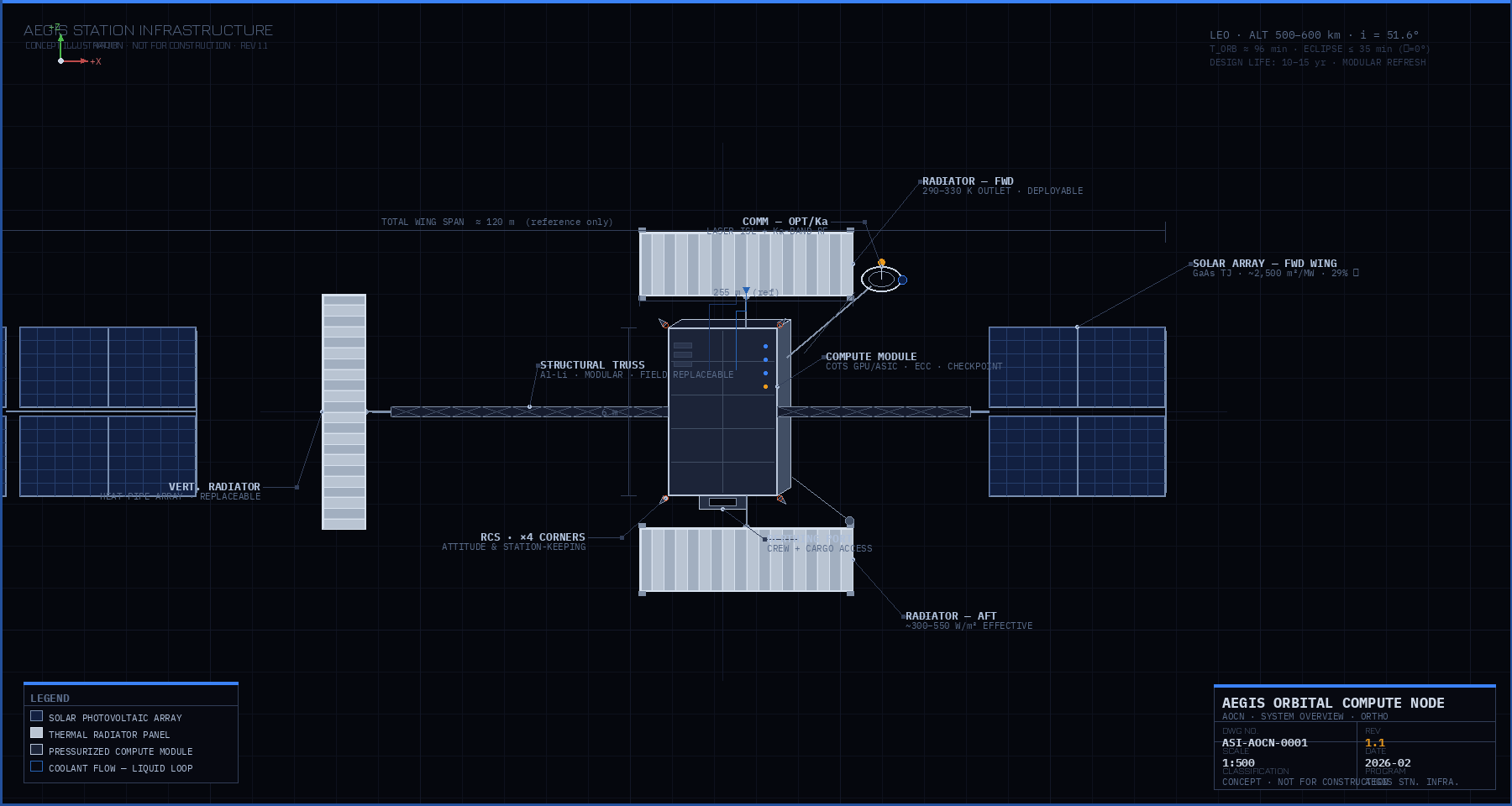
The Aegis Orbital Compute Node (AOCN) is a free-flying compute unit: one megawatt of commercial accelerators in a shielded vault, a fixed solar sheet that faces the sun all year, and pumped-loop radiators that never see it. It runs batch work: model training, large-scale inference, simulation, and the processing of data that is already in orbit. It does not run a cloud. Nothing on it answers a request in milliseconds, and nothing on it needs to.

The node is the unit of scale. Capacity grows by flying more of them, not by making one bigger. Every node is sized, launched, and serviced the same way, and the compute inside is expected to be replaced every three to five years while the power and thermal plant stays.

Why Put Compute in Orbit

The honest case is narrower than the slogans and stronger than the sceptics allow. Three things are true at once.

1. The constraint on Earth is the grid, not the chip

Terrestrial AI capacity is gated by interconnect queues measured in years, by water for cooling, and by siting permits. In orbit none of those exist. Power is not free; it costs launched array mass. But a square metre of array in a dawn-dusk orbit produces about four and a half times the energy of the same square metre on the ground, because it is lit 100 % of the time at full solar constant and needs no storage. The question is whether that buys back the launch cost, and the economics section answers it with a number rather than a mood.

2. Batch work does not need a fast link to Earth

Training a large model is weeks of computation on a dataset that arrives once and a result that leaves once. That is the opposite of a cloud workload. The dataset goes up on launched storage: ten petabytes on enterprise SSDs is under 200 drives and well under half a tonne. Checkpoints and weights come down over optical crosslinks. A dawn-dusk orbit passes a polar ground station on nearly every revolution, so downlink capacity is not the limit. The data section sizes it.

3. Some customers are already in space

Earth-observation constellations downlink raw data they could process in orbit. Cislunar operations, when they exist, will want compute that is seconds away rather than a round trip through Earth. This is the only case with no terrestrial competitor. It is also the smallest market today, which is why AOCN is not designed around it. It is designed so that the same node serves it when it arrives.

Data Path

Dawn-dusk sun-synchronous orbits cross both poles every ~97 minutes. A single high-latitude optical terminal sees the node on most passes; two terminals on different continents cover weather.

Orbit Selection

Rev 1.1 assumed a generic 500–600 km orbit with a 35 % worst-case eclipse and either 2.6 t of battery per megawatt or a throttled duty cycle. The battery figure was cell-level; at a LEO-survivable depth of discharge and pack overhead it is closer to 12 t per node. That is a sizing problem, not a barrier; a node with a battery is buildable. Rev B chooses the orbit that does not need one, because everything downstream gets simpler: a fixed array, a constant sun, one radiator plane, and no charge cycle every orbit. Nothing moves and nothing cycles.

A dawn-dusk sun-synchronous orbit keeps its plane at the day-night terminator all year. The sun sits within about 24° of the orbit normal. Above roughly 620 km the Earth never gets between the node and the sun, at any season. AOCN Rev B baselines 650 km.

• No eclipse, no battery. A small pack for safe-mode only. Compute runs continuously.
• Fixed geometry. The array is a flat sheet in the orbit plane facing the sun; it needs no gimbal. Radiators lie in the plane containing the sun vector and nadir, so their faces look along the velocity vector, never at the sun and only obliquely at Earth. The array shades them as well.
• Ground contact. Both poles every orbit, which is what makes the optical downlink budget work.
• Drag. The array is edge-on to the velocity vector; the radiators are not. About 2,100 m² of ram area at 650 km costs ~13 m/s per year, under 50 kg of xenon per year on electric propulsion. Atomic-oxygen-tolerant radiator coatings are required.
• Radiation. The price of the orbit. A polar orbit crosses the auroral horns and the South Atlantic Anomaly; total dose is several times an ISS-orbit figure. The vault section carries it.

Arrangement

Thermal: Radiator Sizing

At steady state every watt of electrical input becomes heat. Commercial accelerators hold junction temperatures below about 363 K; direct liquid cooling delivers coolant at 305–320 K and returns it 10–15 K warmer. The radiator therefore runs between roughly 330 K inlet and 305 K outlet, a 315 K mean radiating temperature. Rev 1.1 stated 290–330 K; the same range, now pinned to a sizing point.

Two-sided rejection follows the Stefan-Boltzmann law with an emissivity of 0.88. An effective factor of 0.6 covers Earth infrared on the oblique face, view-factor losses between wings, coating degradation, and fin efficiency. With the array shading the wings and no direct solar load, this factor is conservative.

The node rejects 1.2 MW, so the baseline radiator area is ~2,000 m² two-sided, carried as two 50 × 20 m wings on a pumped single-phase loop with redundant pumps and isolable sections. At 6 kg/m² for deployable pumped-loop panels the wings weigh about 12 t. If a future accelerator generation tolerates hotter coolant, the same wings reject more; the plant does not need to change when the trays do.

Power: Solar Array Sizing

Rev 1.1 sized the array at ~2,500 m² per MW from beginning-of-life cell efficiency at normal incidence. That is the number for a new panel pointed perfectly on the day it deploys. The array has to make 1.2 MW on its last day, at its worst sun angle, through a blanket that is not all cells.

Compute Vault and Radiation

Rev 1.1 carried 15–50 t of water and structure as shielding for a compute payload. That is a crew figure applied to electronics. Silicon does not need a storm shelter; it needs a tolerable total dose, a handled upset rate, and a refresh plan.

• Total dose. A 650 km polar orbit delivers on the order of several kilorad per year behind thin aluminium, dominated by South Atlantic Anomaly protons. Commercial accelerators and memory have been shown tolerant into the 10–30 krad range. A vault wall of 10–15 mm aluminium-equivalent cuts the annual dose by a factor of three to five and puts a 3–5 year tray life inside the envelope. That interval already matches the commercial hardware cycle.
• Upsets. Polar and SAA passes raise the single-event rate on unhardened parts. The answer is architectural: ECC memory, frequent checkpointing to the local storage pool, and scheduling that expects a few percent of throughput lost to restarts. This is the open engineering question on the node and the page does not pretend it is closed.
• Geometry. The vault is an unpressurised cylinder, ⌀4 × 10 m, with cold-plated trays on rails so a robotic servicer can swap a tray without breaking the coolant loop. Storage, power conversion, and the loop pumps live in the same shell. Vault structure and shielding together are ~5 t, not 15–50.
• Serviceability. Interfaces are EVA-compatible so a crewed servicing mission is possible, but nothing on the node requires a person. The array blankets and radiator wings are line-replaceable units on the same truss standard.

Mass Budget, 1 MW IT Node

Rev 1.1 carried 40–80 t for 200–500 kW of accelerator. Rev B carries ~65 t for 1,000 kW. The change is not optimism; it is the removal of the water shield and the batteries, and the accounting of compute at the density liquid-cooled racks actually achieve. The refresh cycle relaunches only the 12 t of trays.

Economics: Where It Crosses Over

Both an orbital node and a terrestrial hall buy the same accelerators, and those dominate the bill either way: on the order of $40–50 M per megawatt of current-generation hardware. What differs is the plant around them. A terrestrial AI hall costs roughly $10–15 M per MW to build, plus around $0.6–0.9 M per MW-year in energy. Over a five-year hardware life that is about $15–20 M per MW of plant and power, before the years spent waiting for an interconnect.

The orbital node replaces all of that with launch mass. At 65 t per megawatt:

The crossover sits near $300 per kilogram to sun-synchronous orbit, before counting on-orbit assembly, qualification, and the operations team, which push it lower, and before counting the value of skipping a multi-year grid queue, which pushes it higher. That price does not exist today. It is the stated goal of fully reusable heavy launch, and the point of writing the number down is that it is a launch-price gate, not a technology gate. Everything else on this page is buildable now.

Scaling

Nothing in the node gets easier when it gets bigger. Deployed area, bending modes, pointing disturbance, fault-domain size, and the mass of any single failure all grow faster than the compute they carry. A 1 MW node is already a 90 m sheet with 50 m wings. The unit is fixed and the fleet grows.

• Plane fill. Nodes in the same dawn-dusk plane share ground stations and can crosslink for distributed training. Ten nodes is 10 MW of accelerator in one plane with one ground segment.
• Independent failure. A punctured loop or a lost wing takes out one node, throttled, not a fleet.
• Same servicer. One robotic servicing vehicle and one tray standard cover every node in the plane.
• Lifecycle split. Plant lasts 10–15 years; trays turn over in 3–5. The plant is the asset; the trays are inventory.

Beyond Earth Orbit

The node does not care which body it orbits, but the case does. Around the Moon or Mars there is no advantage until there are customers there, and the Earth link gets worse. Where the case changes is the lunar surface, and only one part of it.

The lunar surface as a heat sink, with the caveat

The daytime surface is not a cold sink. At the equator it reaches ~390 K at noon for two weeks, and regolith is an insulator, so nothing conducts into the ground worth counting. A radiator on the day side of the Moon looks at hot ground and a hot sun for 14 days and then at nothing but darkness for 14 more, with no power.

The polar surface is different. Rim sites near the south pole are lit 80–90 % of the year at grazing angles, and next to them are permanently shadowed floors at 40–100 K. A vertical radiator on a rim, facing the shadowed floor and the cold sky, rejects about 490 W/m² one-sided at 315 K with no Earth infrared and no solar load. Per square metre that is comparable to the orbital wing. The difference is everything around it: no launch of the plant from Earth once regolith structure and local water are available, no deployment mechanisms, radiators that can be built as walls, and the program's own water on site for thermal storage across the short polar nights.

What Changed From Rev 1.1

Technical Reference

The Rev B architecture reference document carries the sizing set above with its bases, the mass budget, the economics table, and the lunar polar variant.